Bayesian Inference Part 1: My Picky Cat Parker.

Introduction
This is the first of two blog posts regarding Bayes’ Theorem and Bayesian Inference and its application in data science. The intention of these posts is simply to introduce and explain these concepts at a very high level. There are a number of thorough resources available that go into these topics in much more detail. The point here is to have some fun with this and potentially show the value of Bayesian thinking when it comes to data science.
This first post is dedicated to one of our two cats. His name is Parker. Our other cat Zoe will get a blog post of her own someday. Don’t worry, I am not playing favorites.
“Get off the damn counter!”
My kids have heard me say that more than once. It was not directed at them, but at our cat, Parker. Parker is known for two things:
- Holding down our beds.
- Jumping up on the counter.
As for the first point, let’s just say that Parker doesn’t like to waste his energy. As for the second, Parker particularly likes to jump on the counter when there is a serving plate with food there.
Consider the following table that shows the frequency that Parker jumps up on the counter when we place food there.
Parker jumping up on the counter vs staying on the floor:
| Jump | Stay |
|---|---|
| 11 | 9 |
(Note: This data was created with a simulated Parker. The actual Parker is resting on our bed and I didn’t want to disturb him.):

A Frequentist Approach
A frequentist approach to this data suggest that there is a slightly better than 50% chance that Parker will jump up on the counter. Running the test over and over to get a bigger sample size would help better nail down the probability that Parker will jump on the counter. Or would it? It turns out that there is more going on here. With a little Bayesian thinking, we can reach a different conclusion. And, in the process, not disturb the sleeping Parker. I’m sure he would approve.
Bayesian Approach: Conditional Probabilities
Let’s say we had access to more information than is shown in the above table. For instance, what if we know that Parker is particularly fond of salmon. Let’s take a look at that data again and this time take into account the type of food that is sitting on the counter:
Conditional results for Parker jumping up on the counter:
| Food on Counter | Jump | Stay |
|---|---|---|
| Salmon | 9 | 1 |
| Not Salmon | 2 | 8 |
Intuition tells us, based on this data, that if we put salmon on the counter it is more likely that Parker will jump up there than if there is some other kind of food involved. We can use Bayes’ Theorem to get a sense for what the probability is if we put salmon on the counter.
Bayes’ Theorem looks like this:
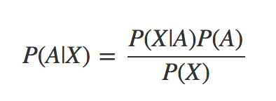
Let’s use this theorem and the table that we have above to see if we can compute the probability that Parker will jump on the counter the next time we serve salmon.
P(A|B) This is the probability that Parker will jump on the counter given that we are serving salmon. It is also called the “posterior probability”. This is what we are trying to figure out.
P(B|A) This the probability that we served salmon given that Parker jumped up on the counter. This would be 9/11 = .8182
P(A) This is the probability of the outcome occurring without knowledge of new data. It is reflected in the first table, or 11/20 = .55
P(B) This is the probability of the evidence arising. For us it is 10/20 because we served salmon 10 out of 20 times. Plugging those numbers into the equation above we get:
P(A|B) = (0.8182 * 0.55) / 0.5 = 0.9
Now, look back at the data table above. Note that Parker jumped up on the counter 9 out of 10 times when we served salmon. So, based on our data, we can see that the probability of Parker jumping up on the counter when we serve salmon is 9/10 or .9. Bayes’ Theorem gives us the exact same answer.
In this case we really didn’t need Bayes’ Theorem to calculate the results. However what if we didn’t have a nice simple data table like the one above.
A More Complicated Example
(Taken from Introduction to Probability and Statistics, Second Edition by J.S. Milton and Jesse C. Arnold, McGraw-Hill Publishing 1990. ISBN: 0-07-042353-9)
A test has ben developed to detect a particular type of arthritis in individuals over 50 years old. From a national survey, it is known that approximately 10% of the individuals in this age group suffer from this form of arthritis. The proposed test was given to individuals with confirmed arthritic disease, and a correct test result was obtained in 85% of the cases. When the test was administered to individuals of the same age group who were known to be free of the disease, 4% were reported to have the disease. What is the probability that an individual has this disease given that the test indicates its presence.
So, from the above, we know:
P(A|B) This is the posterior probability and is what we are looking for. The probability that an individual has the disease given that the test says they do.
P(A) = the probability of having the disease = .1
P(B|A) = the probability of the test being positive given the disease is present = .85
So far, these have all been easy. They are just taken directly from the problem. Now for the tricky one…
P(B) = the probability that the test is positive and the disease is present plus the probability that the test is positive but the disease is NOT present. (We annotate not with a “~”)…
 =
=

Substituting this all back into Bayes’ Theorem we have

It is somewhat remarkable that we can only be around 70% confident based on a test that is 85% accurate!
Conclusion
In this short blog post we explored using Bayes’ Theorem to arrive at conditional probabilities. Check out my next blog post where we will explore using a technique called Bayesian Inference on tweets by President Trump.
It is sure to be entertaining!
More Resources
For this blog post, I borrowed heavily from a number of resources. I would encourage anyone interested in learning more about Bayesian techniques to check them out.
- http://www.kevinboone.net/bayes.html
- https://www.countbayesie.com/blog/2015/2/18/bayes-theorem-with-lego
- https://www.math.hmc.edu/funfacts/ffiles/30002.6.shtml
- https://www.analyticsvidhya.com/blog/2016/06/bayesian-statistics-beginners-simple-english/
- https://www.coursera.org/learn/mcmc-bayesian-statistics/home/welcome